In a malware galaxy far away: Visualizing malware clusters with ssdeep and plotly

20 Apr 2025

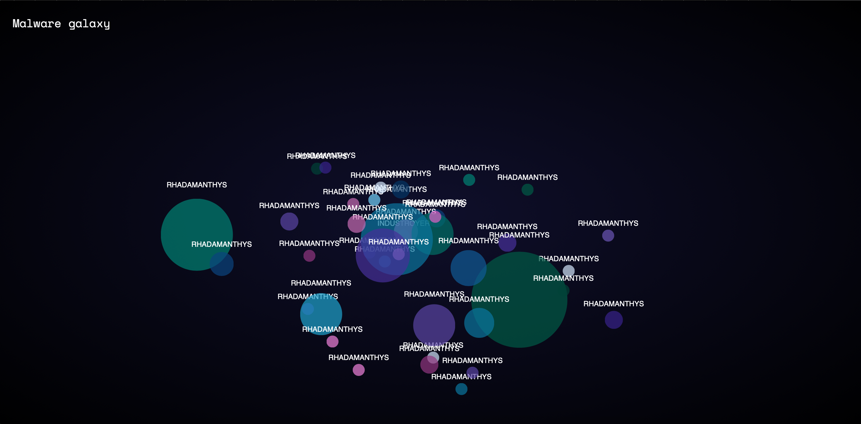
tl;dr; Grouping malware based on similarity in behavior or structure is a tried-and-true technique in Threat Intelligence. This blog post shows how fuzzy hashing via ssdeep, combined with Multi-Dimensional Scaling (MDS), can be used to cluster — and more importantly, visualize — malware associated with threat actors. And it looks like this (click the image for a live example):

With traditional hashes like SHA256 or MD5, the entire hash changes if you modify even a single byte in a file. Super handy if you want to know whether a file is an exact match, but absolutely useless if you’re looking for files that are slightly different. Think recompilations, some extra obfuscation, or a small tweak in the code.

And that’s exactly why fuzzy hashing is often used in malware analysis. One of the most well-known tools for this is ssdeep. Instead of returning a fixed hash, ssdeep generates a kind of fingerprint based on the context and structure of a file. That means you’re no longer just asking “Is this the exact same file?” but also “How similar is this to something we’ve seen before?” — with a score between 0 and 100. Way more useful when you’re looking for variants rather than exact copies.

Take for example this file with the following hashes:

MD5: 583ec7348c3817d757ee5844f665f293
SHA256: ff457cc4b90c5c28ce85107b386fddfb4a7dd42c9c401a9598a46ce36b43a5b5
ssdeep: 12:wiVUXxCWEUbNI9kxwAUIySKxWHUWyFULPCUNoeVUb6UJxRI4qKAUKJeUwx7+cAUd:rmv5bNIqcCKxzeHNU3Z1xlmv5goHA

Using this fuzzy hash, you can calculate how similar it is to other files. Both this file and this file are tagged as Mirai shell script droppers on MalwareBazaar. Whether they’re actually similar, you can calculate using this function:

Example:

# Usage: ssdeep.compare(hash1, hash2)
ssdeep.compare(
    "12:wiVUXxCWEUbNI9kxwAUIySKxWHUWyFULPCUNoeVUb6UJxRI4qKAUKJeUwx7+cAUd:rmv5bNIqcCKxzeHNU3Z1xlmv5goHA",
    "12:eiV+mxCWE+QNI9kxwA+5ySKxWH+exRI4qKA+Svq+UPC+2oeV+DJe+vx7+cA+xy9T:h7mNIqYKxS1x6wsZa8v"
)

The ssdeep.compare function returns a score between 0 (completely different) and 100 (nearly identical). In this example, the files are 55% similar. They’re both shell scripts, so that’s easy to verify. Both do a lot of wget and chmod — the score seems pretty legit. So now you can spot not just exact duplicates, but also closely related variants from the same malware family.

Sounds ideal — but not quite, for a couple of reasons:

It’s sensitive to packers or payload encryption
The order and structure of content affect the score

Still, in situations where you’re trying to group possible malware variants from the same threat actor, it can reveal valuable insights. In the rest of this post, I’ll show how to use tagged APT samples to create a visualization based on their ssdeep hash and MDS clustering.

Fetching ssdeep info from MalwareBazaar

Step one is collecting relevant malware to cluster. In this example, I picked two APT groups (I saw two bears…) and looked up related malware on Malpedia, defining them in apt_groups. Then, for each family, I fetch all samples from MalwareBazaar tagged with those names and extract their ssdeep hashes:

apt_groups = {
    "apt28": ["xagent", "komplex", ...],
    "apt29": ["beatdrop", "boombox", ...]
}

for apt, tools in apt_groups.items():
    for tool in tools:
        data = get_malware_bazaar(apt, tool)

The get_malware_bazaar() function uses the MalwareBazaar API to pull files based on a tag. The data is saved into a simple SQLite database:

class Signature(db.Model):
    id = db.Column(db.Integer, primary_key=True)
    filename = db.Column(db.String(255))
    filetype = db.Column(db.String(50))
    signature_name = db.Column(db.String(255))
    actor = db.Column(db.String(50))
    sha256 = db.Column(db.String(64), unique=True)
    ssdeep = db.Column(db.String(255))
    date = db.Column(db.DateTime)

def get_malware_bazaar(actor, signature_name):
    headers = {'API-KEY': [API_KEY_HERE]}
    data = {'query': 'get_taginfo', 'tag': signature_name}

    response = requests.post('https://mb-api.abuse.ch/api/v1/', headers=headers, data=data)
    list_data = response.json()

    if 'data' not in list_data:
        return

    with app.app_context():
        for item in list_data['data']:
            if not Signature.query.filter_by(sha256=item['sha256_hash']).first():
                signature = Signature(
                    filename=item['file_name'],
                    filetype=item['file_type'],
                    actor=actor,
                    signature_name=signature_name,
                    sha256=item['sha256_hash'],
                    ssdeep=item['ssdeep'],
                    date=datetime.strptime(item['first_seen'], '%Y-%m-%d %H:%M:%S')
                )
                db.session.add(signature)
        db.session.commit()

This script regularly checks if there are new samples tagged with the names we’ve defined. The result: a SQLite database with rows containing the SHA256 (for deduplication), the ssdeep hash, and the threat actor based on Malpedia.

From hashes to distance matrix

With the ssdeep hashes, you can now compute distances and store them in a matrix. When comparing all hashes using ssdeep.compare and grouping those that score above a certain threshold (here: 75%), you get this snippet. A score above 75% is considered a cluster:

num_files = len(files)
distance_matrix = np.zeros((num_files, num_files))
clusters = []

for i in range(num_files):
    cluster_found = False
    for cluster in clusters:
        similarity = ssdeep.compare(hashes[i], hashes[cluster[0]])
        if similarity >= 75:
            cluster.append(i)
            cluster_found = True
            break
    if not cluster_found:
        clusters.append([i])

Then we build the distance matrix based on compare output, giving extra weight to matches with the same threat actor or tool name. You could just use raw similarity, but in the example below I’ve bucketed them a bit:

0 (if similarity ≥ 75%)
0.25 (same threat actor or signature)
raw similarity
1 (max distance)

for i in range(num_files):
    for j in range(num_files):
        if i != j:
            similarity = ssdeep.compare(hashes[i], hashes[j])
            if similarity >= 75:
                distance_matrix[i, j] = 0
            elif similarity > 0:
                distance_matrix[i, j] = similarity
            elif files[i] == files[j] or apts[i] == apts[j]:
                distance_matrix[i, j] = 0.25
            else:
                distance_matrix[i, j] = 1
        else:
            distance_matrix[i, j] = 0

Translating the distance matrix into points with MDS

Once every sample has a distance calculated to every other sample, you get a big distance matrix. Problem: it’s not easily interpretable visually, especially with dozens or hundreds of samples.

That’s where Multi-Dimensional Scaling (MDS) comes in. It projects the distances between objects into lower-dimensional space (like 2D or 3D), while preserving their relative relationships. The result is a plot where similar samples cluster together and unrelated ones are far apart. Samples with identical ssdeep hashes appear as a single larger dot — cluster size corresponds to number of identical hashes.

from sklearn.manifold import MDS
mds = MDS(n_components=2, dissimilarity="precomputed", random_state=42)
mds_results = mds.fit_transform(distance_matrix)

# Prepare data for Plotly
plot_data = {
    "x": [],
    "y": [],
    "text": [],
    "size": []
}

for cluster in clusters:
    if len(cluster) > 1:
        x = mds_results[cluster, 0].mean()
        y = mds_results[cluster, 1].mean()
        text = files[cluster[0]].upper()
        size = len(cluster) * 10

        plot_data["x"].append(x)
        plot_data["y"].append(y)
        plot_data["text"].append(text)
        plot_data["size"].append(size)

Visualizing with Plotly

Now the fun part: visualizing the distance matrix using Plotly. Plotly is an open-source visualization library in Python (also in JS and R), that creates interactive charts and dashboards. Unlike static visualizations like matplotlib, Plotly uses web tech (HTML, JS, D3.js), enabling zooming, hovering, and clicking.

You can also color and label clusters, like so:

def cluster_plotly(plot_data, clusters):
    fig = go.Figure()
    space_colors = ['#015a46', '#034237', ...]

    num_points = len(plot_data["x"])

    for idx, cluster in enumerate(clusters):
        if isinstance(cluster, list):
            valid_indices = [i for i in cluster if 0 <= i < num_points]
            x = [plot_data["x"][i] for i in valid_indices]
            y = [plot_data["y"][i] for i in valid_indices]
            text = [plot_data["text"][i] for i in valid_indices]
            size = [plot_data["size"][i] for i in valid_indices]
        else:
            if 0 <= cluster < num_points:
                x = [plot_data["x"][cluster]]
                y = [plot_data["y"][cluster]]
                text = [plot_data["text"][cluster]]
                size = [plot_data["size"][cluster]]
            else:
                continue
        print(f"Cluster {idx}: {cluster}")

Result

By using ssdeep hashes like this for clustering and visualization, you can discover interesting patterns — like new malware families or behavioral trends over time. Right now, the app pulls from a limited sample set, and thanks to caching the plotting is quite fast.

However, when working with massive datasets, this approach isn’t optimal in terms of space & time (hello, throwback to Data Structures course). Also, ssdeep alone doesn’t give the best overview possible. In such cases, it’s better to combine multiple techniques — like YARA hits or reused IoCs — for a more complete picture.

Live application